
hash tables - I
Hey, everyone! We're going to talk about one of the most remarkable data structure of all times, Hash Tables.
What is a Hash table?
A Hash table (HT) is a data structure that provides a mapping from keys to values using a technique called hashing.
| Key (name) | Value (fav color) | |
|---|---|---|
| "Tony" | → | "red" |
| "Steve" | → | "blue" |
| "Natasha" | → | "black" |
| "Peter" | → | "red" |
We refer to these as key-value pairs. Keys must be unique, but values can be repeated. HTs are often used to track item frequencies. For example, number of times a word appears in the given text.
I parsed Shakespeare's Romeo and Juliet (ignoring case) and obtained the following frequency table:
| Key (word) | Value (frequency) | |
|---|---|---|
| "'tis" | → | 40 |
| "a" | → | 461 |
| "all" | → | 84 |
| "and" | → | 84 |
| "and," | → | 30 |
| "as" | → | 156 |
| "be" | → | 196 |
| ... | ... | ... |
What is a hash function?
To be able to understand, how a mapping is constructed between key-value pairs we first need to talk about hash functions.
A hash function H(x) that maps a key 'x' to a whole number in a fixed range. For example, H(x) = (x² - 6x + 9) mod 10 maps all integer keys to the range [0,9]
- H(4) = (16 - 24 + 9) mod 10 = 1
- H(8) = (64 - 48 + 9) mod 10 = 5
- H(0) = (0 - 0 + 9) mod 10 = 9
- H(-7) = (49 + 42 + 9) mod 10 = 0
and so on.
We can also define hash functions for arbitrary objects like string, lists, tuples, multi data objects, etc.
For a string s, let H(s) be a hash function defined below where ASCII(x) returns the ASCII value of the character x. (For more check out ASCII TABLE)
function H(s):
  sum := 0
  for char in s:
    sum = sum + ASCII(char)
  return sum mod 50

/*
* H("BB") = (66 + 66) mod 50 = 32
* H("") = (0) mod 50 = 0
* H("ABC") = (65 + 66 + 67) mod 50 = 48
* H("Z") = (90) mod 50 = 40
*/
These are certain arbitrary hash function, we will get to some sophisticated hash functions later in the post.
Properties of hash functions
If H(x) = H(y) then objects x and y might be equal, but if H(x) != H(y) then x and y are certainly not equal.
This might help speed things up in object comparisons. This means that instead of comparing x and y directly a smarter approach is to first compare their hash values, and only if the hash values match do we need to explicitly compare x and y.
Consider the problem of trying to determine if two very large files have the same contents.
If we precomputed H(file1) and H(file2) first we should compare those hash values, since comparing hash values is O(1)! If possible, we do not want to open either of the files directly. Comparing their contents can be very slow, although we may have to if their hashes are equal.
NOTE: Hash functions for files are more sophisticated than those used for hashtables. Instead for files we use what are called cryptographic hash functions also called checksums.
A hash function H(x) must be deterministic.
This means that if H(x) = y then H(x) must always produce y and never another value.
Example of a non-deterministic hash function:
counter := 0
function H(x):
  counter = counter + 1
  return (x + counter) mod 13
The first time called H(2) = 3, but if called again H(2) = 4
We try very hard to make uniform hash functions to minimize the number of hash collisions.
A hash collision is when two objects x, y hash to the same value (i.e. H(x) = H(y)).
We are now able to answer a central question about the types of keys we are allowed to use in our hashtable:
Q: What makes a key of type T hashable ?
Since we are going to use hash functions in the implementation of our hash table we need our hash functions to be deterministic. To enforce this behaviour, we demand that the keys used in our hash table are immutable data types. Hence, if a key of type T is immutable, and we have a hash function H(k) defined for all keys k of type T then we say a key of type T is hashable.
How does a Hash Table Work?
Ideally we would like to have a very fast insertion, lookup and removal time for the data we are placing within our hash table.
Remarkably, we can achieve all this in O(1)* time using a hash function as a way to index into a hash table.
The constant time behaviour attributed to hash tables is only true if you have a good uniform hash function!
Think of the hash table as an indexable block of memory (an array) and we can only access its entries using the value given to us by our hash function H(x). Suppose we're inserting (integer, string) key-value pairs into the table representing rankings of users to their usernames from an online programming competition and we're using the hash function:
H(x) = x² + 3 mod 10
To insert the following key-value pairs: (3, "tourist"), (1, "errichto"), (5, "rpuneet") and others, we hash the key (the rank) and find out where it goes in the table.
- H(3) = (3² + 3) mod 10 = 2
- H(1) = (1² + 3) mod 10 = 4
- H(5) = (5² + 3) mod 10 = 8
- H(10) = (10² + 3) mod 10 = 3
- H(32) = (32² + 3) mod 10 = 7
To lookup which user has rank r we simply compute H(r) and look inside the hashtable!
If we keep on inserting elements, we're bound to have a collision. So a question arises:
Q: What do we do if there is a hash collision?
For example, users with ranks 2 and 8 hash to the same value, i.e. 7!!
We use one of many hash collision resolution techniques to handle this, the two most popular ones are separate chaining and open addressing.
Separate Chaining deals with hash collisions by maintaining a data structure (usually a linked list) to hold all the different values which hashed to a particular value.
Open Addressing deals with hash collisions by finding another place within the hash table for the object to go by offsetting it from the position to which it hashed to.
Complexity
The time complexity of hash tables is actually pretty remarkable.
| Operation | Average | Worst |
|---|---|---|
| Insertion | O(1)* | O(n) |
| Removal | O(1)* | O(n) |
| Search | O(1)* | O(n) |
* The constant time behaviour attributed to hash tables is only true if you have a good uniform hash function!
Separate Chaining
As I mentioned earlier, Separate Chaining is one of many strategies to deal with hash collisions by maintaining a data structure (usually a linked list) to hold all the different values which hashed to a particular value.
NOTE: The data structure used to cache the items which hashed to a particular value is not limited to a linked list. Some implementations use one or a mixture of: arrays, binary trees, self-balancing trees and etc.
Linked List Separate Chaining Insertion and Lookup
Suppose we have a hash table that will store (name, age) key-value pairs and we wish to insert the following entries:
| Name | Age | Hash |
|---|---|---|
| Will | 21 | 3 |
| Leah | 18 | 4 |
| Rick | 61 | 2 |
| Rai | 25 | 1 |
| Lara | 34 | 4 |
| Ryan | 56 | 1 |
| Finn | 21 | 3 |
| Mark | 10 | 4 |
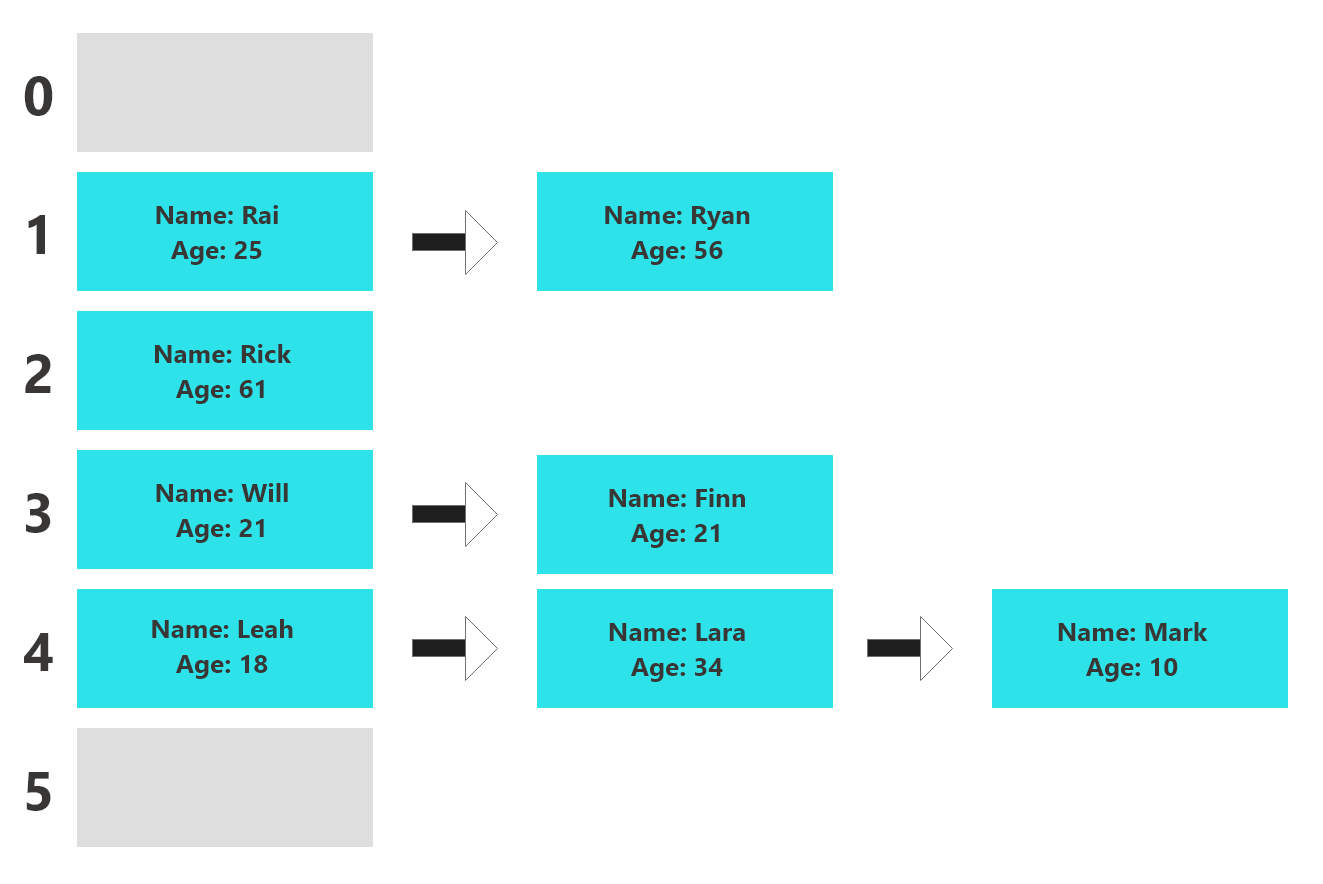
For lookups, suppose we need to find age of "Ryan", we hash the key "Ryan" to obtain the value (index) 1. After this scan the 1 bucket for the key "Ryan".
It may happen that the value you are looking for does not exist in bucket the key hashed to in which case the item does not exist in the HT.
Q: How do I maintain O(1) insertion and lookup time complexity once my HT gets really full and I have long linked list chains?
Once the HT contains a lot of elements you should create a new HT with a larger capacity and rehash all the items inside the old HT and disperse them throughout the new HT at different locations.
Q: How do I remove key-value pairs from my HT?
Apply the same procedure as doing lookup for a key, but this time instead of returning the value associated with the key, remove the node in the linked list data structure.
Q: Can I use another data structure to model the bucket behaviour required for the separate chaining method?
Of course! Common data structures used instead of a linked list include: arrays, binary trees, self balancing trees, etc. You can even go with a hybrid approach like Java's HashMap.
Here's my implementation of Hash Tables using Separate Chaining in C++:
/*
  An implementation of a hash-table
  using separate chaining with a linked list.

  @author: Gyan Prakash Karn, karngyan@gmail.com
*/

#include<iostream>
#include<limits>
#include<vector>
#include<algorithm>
#include<string>
#include<cfloat>

template<class K, class V>
class Entry {
public:
  std::hash<K> H;
  long long int hash;
  K key;
  V value;

  template<class A, class B>
  Entry(A k, B v) {
    key = k;
    value = v;
    hash = H(key);
  }

  bool operator== (const Entry & other) {
    if (hash != other.hash) return false;
    return key == other.key;
  }
};

template<class K, class V>
class HashTableSeparateChaining {
  constexpr static int DEFAULT_CAPACITY = 3;
  constexpr static double DEFAULT_LOAD_FACTOR = 0.75;
  double maxLoadFactor;
  int capacity, threshold, sze = 0;
  std::vector<std::vector <Entry<K, V>>> table;
  std::hash<K> H;

public:
  HashTableSeparateChaining(int cap, double mLF) {
    maxLoadFactor = mLF;
    capacity = cap;
    threshold = (int) (capacity * maxLoadFactor);
    table.clear();
    table.resize(capacity);
  }

  HashTableSeparateChaining() : HashTableSeparateChaining(DEFAULT_CAPACITY, DEFAULT_LOAD_FACTOR){}

  int size() { return sze; }
  bool empty() { return sze == 0; }

  bool hasKey(K key) {
    int bucketIndex = normalizeIndex(H(key));
    return bucketSeekEntry(bucketIndex, key) != NULL;
  }

  void insert(K key, V value) {
    Entry<K, V> newEntry(key, value);
    int bucketIndex = normalizeIndex(newEntry.hash);
    bucketInsertEntry(bucketIndex, newEntry);
  }

  V* get(K key) {
    int bucketIndex = normalizeIndex(H(key));
    Entry<K, V> *entry = bucketSeekEntry(bucketIndex, key);
    if (entry != NULL) return &(entry->value);
    return NULL;
  }

  V* remove(K key) {
    int bucketIndex = normalizeIndex(H(key));
    return bucketRemoveEntry(bucketIndex, key);
  }

private:
  int normalizeIndex(int keyHash) {
    return (keyHash & 0x7FFFFFFF) % capacity;
  }
  // ... bucket operations omitted for brevity
};

int main() {
  HashTableSeparateChaining<std::string, std::string> map;
  map.insert("tourist", "red");
  map.insert("rpuneet", "purple");
  map.remove("rpuneet");
  return 0;
}
Open Addressing
When using open addressing as a collision resolution technique the key-value pairs are stored in the table (array) itself as opposed to a data structure like in separate chaining.
Load factor = (items in table) / (size of table)
The O(1) constant time behaviour attributed to hash tables assumes the load factor (α) is kept below a certain fixed value. This means once α > threshold we need to grow the table size (ideally exponentially, e.g. double).
There are infinite amount of probing sequences you can come up with:
Linear Probing: P(x) = ax + b, where a,b are constants
Quadratic Probing: P(x) = ax² + bx + c, where a, b, c are constants
Double Hashing: P(k, x) = x*H₂(k), where H₂(k) is a secondary hash function.
Pseudo random number generator: P(k, x) = x*RNG(H(k), x), RNG is a random number generator function seeded with H(k).
General insertion method for open addressing on a table of size N:
x := 1
keyHash := H(k)
index := keyHash

while table[index] != null:
  index = (keyHash + P(k, x)) mod N
  x = x+1

insert (k, v) at table[index]
Chaos with cycles
Most randomly selected probing sequences modulo N will produce a cycle shorter than the table size. This becomes problematic when you are trying to insert a key-value pair and all the buckets on the cycle are occupied because you will get stuck in an infinite loop!
In general the consensus is that we avoid it altogether by restricting our domain of probing functions to those which produce a cycle of exactly length N.
Notice that open addressing is very sensitive to the hashing and probing function. This is not something one has to worry about if they're using separate chaining as a collision resolution method.
Hope you liked it! I'll cover more about Probing Functions and their source code in the next part of the blog.